A while ago i had tried my hand at various video tutorials. Following post is a starting point one of the basic videos that i made.
The videos are targeted for the absolute beginners. The post supports by displaying some of the content that is there in the video format. The post is for the readers who want to have a quick read and get an overall idea about the video.
I hope you enjoy the videos. Probably will make some more on specific topics when i find time.
Programming with Matlab
Timstamps
In this post
Algorithms
Algorithm is need to frame a program that will solve some problem.
- Algorithms is an ordered sequence of precisely defined instructions that performs some task in a finite amount of time.
- An ordered sequence means that the instructions can be numbered
- An algorithm often must have the ability to alter the order of its instructions using what is called a control structure.
- There are three categories of algorithmic operations:
- Sequential operations: These instructions are executed in order.
- Conditional operations: These control structures first ask a question to be answered with a true/false answer and then select the next instruction based on the answer.
- Iterative operations (loops):. These control structures repeat the execution of a block of instructions.
- Not every problem can be solved with an algorithm, and some potential algorithmic solutions can fail because they take too long to find a solution.
Structured Programming
Structured programming is a technique for designing programs in which a hierarchy of modules is used, each having a single entry and a single exit point, and in which control is passed downward through the structure without unconditional branches to higher levels of the structure. These modules can be built-in or user-defined functions.
An unfortunate result of the goto statement was confusing code, called spaghetti code, composed of a complex tangle of branches.
Structured programming, if used properly, results in programs that are easy to write, understand, and modify.
The advantages of structured programming are shown here:
- Structured programs are easier to write because the programmer can study the overall problem first and deal with the details later .
- Modules (functions) written for one application can be used for other applications (this is called reusable code).
- Structured programs are easier to debug because each module is designed to perform just one task, and thus it can be tested separately from the other modules.
- Structured programming is effective in a teamwork environment because several people can work on a common program, each person developing one or more modules.
- Structured programs are easier to understand and modify, especially if meaningful names are chosen for the modules and if the documentation clearly identities the module’ s task.
Top Down Design
A method for creating structured programs is top-down design, which aims to describe a program’s intended purpose at a very high level initially and then partition the problem repeatedly into more detailed levels, one level at a time, until enough is understood about the program structure to enable it to be coded.
A structure chart displays the organization of a program without showing the details of the calculations and decision processes. For example, we can create program modules using function les that do speci c, readily identi able tasks. Larger programs are usually composed of a main program that calls on the modules to do their specialized tasks as needed. A structure chart shows the connection between the main program and the modules.

This is an example where a game, say, Tic-Tac-Toe is made. There is a module to allow the human player to input a move, a module to update and display the game grid, and a module that contains the computer’s strategy for selecting its moves.
Flowcharts are useful for developing and documenting programs that contain conditional statements, because they can display the various paths (called branches) that a program can take, depending on how the conditional statements are executed.
Relational Operators
Matlab has 6 relational operators that can be used with an array.
| Relational Operator |
| < Less than |
| > Greater than |
| <= Less than or equal to |
| >= Greater than or equal to |
| == Equal to |
| ~= Not Equal to |
>> x = [6,3,9]
>> y = [14,2,9]
>> z = (x < y)
z =
	1 0 0
>> z = (x ~= y)
z =
	1 1 0
>> z = (x > 8)
z =
	0 0 1
Matlab has 5 logical operators which are sometimes called boolean operators. These perform element by element operation.
| Logical Operators | Definition |
| ~ NOT | ~A returns an array of the same dimension as A; the new array has 1s where A is 0 and 0s where A is nonzero. |
| & AND | A & B returns an array of the same dimension as A and B; the new array has 1s where both A and B have nonzero elements and 0s where either A or B is 0. |
| | OR | A | B returns an array of the same dimension as A and B; the new array has 1s where at least one element in A or B is nonzero and 0s where A and B are both 0. |
| && ShortCircuit AND | Operator for scalar logical expressions. A && B returns true if both A and B evaluate to true, and false if they do not. |
| || ShortCircuit OR | Operator for scalar logical expressions. A || B returns true if either A or B or both evaluate to true, and false if they do not. |
Conditional If and Else Statement
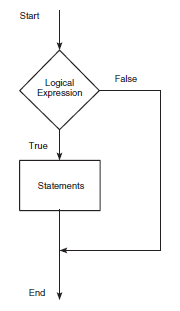
The if statement’s basic form is
if logical expression
statements
end
Every if statement must have an accompanying end statement. The end statement marks the end of the statements that are to be executed if the logical expression is true. A space is required between the if and the logical expression, which may be a scalar, a vector, or a matrix.

if logical expression 1
	statement group 1
end

if x >= 0
	y = sqrt(x)
End

z = 0;w = 0;
if (x >= 0)&(y >= 0)
	z = sqrt(x) + sqrt(y)
	w = sqrt(x*y)
end
The code above can be explained as follows. Here in code, we have an input x we have to do square root for the same. We can add input check like if x >= 0 then and only then we do the dquare rooting. So same has been demonstrated here. We have if x >= 0 then we have output y as square root of x.
In case where input x is negative program will take no action. The logical expression may be a compound expression; the statements may be a single command or a series of commands separated by commas or semicolons or on separate lines. For example, if x and y have scalar values,
When more than one action can occur as a result of a decision, we can use the else and elseif statements along with the if statement. The basic structure for the use of the else statement is:

if logical expression
	statement group 1
else
	statement group 2
end

>> if x >= 0
	y = sqrt(x)
>> else
	y = exp(x) - 1
>> end
The above code example can be exapnded as follows: Suppose that for x >= 0 y = squareroot(x) and for negative values of x y = exp(x) – 1. When the test, if logical expression, is performed, where the logical expression may be an array, the test returns a value of true only if all the elements of the logical expression are true!
The else statement can be used with elseif to create detailed decisionmaking programs

if x > 10
	y = log(x)
elseif x >= 0
	y = sqrt(x)
else
	y = exp(x) - 1
end
Suppose for x > 10 y=ln(x) , for x in between 0 and 10 y is sqrt(x) and for negative value of x y = exp(x) – 1. The statements shown above will compute the same thing y if x already has a scalar value.
Decision structures may be nested; that is, one structure can contain another structure, which in turn can contain another, and so on. Indentations are used to emphasize the statement groups associated with each end statement.
For Loop
A loop is a structure for repeating a calculation a number of times. Each repetition of the loop is a pass. MATLAB uses two types of explicit loops: the for loop, when the number of passes is known ahead of time, and the while loop, when the looping process must terminate when a specified condition is satisfied and thus the number of passes is not known in advance.
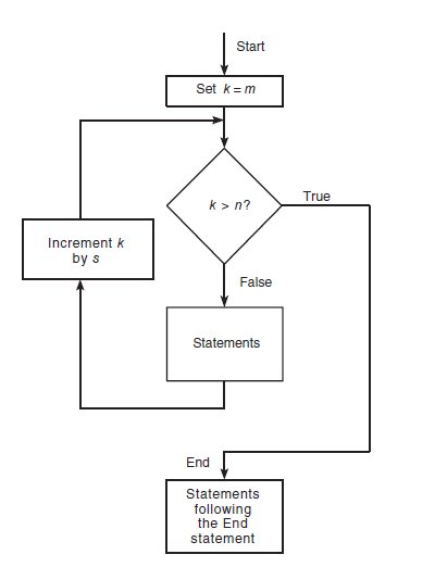
for loop variable=m:s:n
	statements
End

>> for x = 0:2:10, y = sqrt(x), end

>> for k = 5:10:35
	x = k^2
>> end
However, the form written in a single line is less readable than the structured one. The usual practice is to indent the statements to clarify which statements belong to the for and its corresponding end and thereby improve readability.
While Loop
The while loop is used when the looping process terminates because a specified condition is satisfied, and thus the number of passes is not known in advance.
>> while logical expression
	statements
>> End


>> x = 5;
>> while x < 25
	disp(x)
	x = 2*x - 1;
>> end
The results displayed by the disp statement are 5, 9, and 17. The loop variable x is initially assigned the value 5, and it has this value until the statement x = 2*x – 1 is encountered the first time. The value then changes to 9. Before each pass through the loop, x is checked to see whether its value is less than 25. If so, the pass is made. If not, the loop is skipped and the program continues to execute
any statements following the end statement.
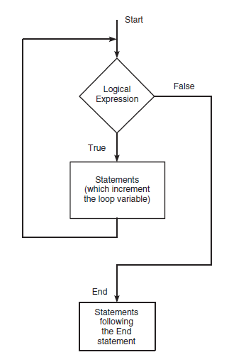
A principal application of while loops is when we want the loop to continue as long as a certain statement is true. Such a task is often more difficult to do with a for loop. The typical structure of a while loop follows.
MATLAB first tests the truth of the logical expression. Aloop variable must be included in the logical expression. For example, x is the loop variable in the statement while x < 25. If the logical expression is true, the statements are executed. For the while loop to function properly, the following two conditions must occur:
- The loop variable must have a value before the while statement is executed.
- The loop variable must be changed somehow by the statements.
The statements are executed once during each pass, using the current value of the loop variable. The looping continues until the logical expression is false.
Each while statement must be matched by an accompanying end. As with for loops, the statements should be indented to improve readability. we may nest while loops, and we may nest them with for loops and if statements
Sometimes when we miss out certain condition or some thing happens that our specified condition never meets then the while loop goes into an infinite loop. If such a loop occurs, press Ctrl-C to stop it.
Break and Continue Statements
We can jump or skip loop iteration using these two statements. The break command, which terminates the loop but does not stop the entire program, can be used for this purpose.
for k = 1:10
	x = 50 - k^2;
	if x < 0
		break
	end
	y = sqrt(x)
end
% The program execution jumps to here
% if the break command is executed.
However, it is usually possible to write the code to avoid using the break command. The break statement stops the execution of the loop. There can be applications where we want to not execute the case producing an error but continue executing the loop for the remaining passes. We can use the continue statement to do this. The continue statement passes control to the next iteration of the for or while loop in which it appears, skipping any remaining statements in the body of the loop. In nested loops, continue passes control to the next iteration of the for or while loop enclosing it.
For example, the following code uses a continue statement to avoid computing the logarithm of a negative number.
x = [10,1000,-10,100];
y = NaN*x;
for k = 1:length(x)
	if x(k) < 0
		continue
	end
	kvalue(k) = k;
	y(k) = log10(x(k));
end
Switch Structure
The switch structure provides an alternative to using the if, elseif, and else commands. Anything programmed using switch can also be programmed using if structures. However, for some applications the switch structure is more readable than code using the if structure. The syntax is:
switch input expression (scalar or string)
case value1
statement group 1
case value2
statement group 2
.
.
.
otherwise
statement group n
end
The input expression is compared to each case value. If they are the same, then the statements following that case statement are executed and processing continues with any statements after the end statement. If the input expression is a string, then it is equal to the case value if strcmp returns a value of 1 (true). Only the rst matching case is executed. If no match occurs, the statements following the otherwise statement are executed. However, the otherwise statement is optional. If it is absent, execution continues with the statements following the end statement if no match exists. Each case value statement must be on a single line. For example, suppose the variable angle has an integer value that represents an angle measured in degrees from North. The following switch block displays the point on the compass that corresponds to that angle.
switch angle
case 45
disp(‘Northeast’)
case 135
disp(‘Southeast’)
case 225
disp(‘Southwest’)
case 315
disp(‘Northwest’)
otherwise
disp(‘Direction Unknown’)
end
Example – Application to Simulation
Simulation is the process of building and analyzing the output of computer programs that describe the operations of an organization, process, or physical system. Such a program is called a computer model. Simulation is often used in operations research, which is the quantitative study of an organization in action, to find ways to improve the functioning of the organization. Simulation enables engineers to study the past, present, and future actions of the organization for this purpose. Operations research techniques are useful in all engineering fields. Common examples include airline scheduling, traffic flow studies, and production lines. The MATLAB logical operators and loops are excellent tools for building simulation programs.
Problem
As an example of how simulation can be used for operations research, consider the following college enrollment model. A certain college wants to analyze the effect of admissions and freshman retention rate on the college’s enrollment so that it can predict the future need for instructors and other resources. Assume that the college has estimates of the percentages of students repeating a grade or leaving school before graduating. Develop a matrix equation on which to base a simulation model that can help in this analysis.
Solution
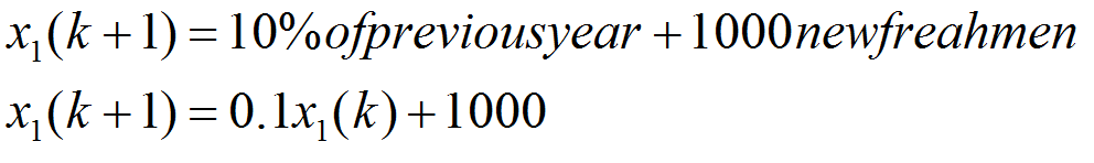
Suppose that the current freshman enrollment is 500 students and the college decides to admit 1000 freshmen per year from now on. The college estimates that 10 percent of the freshman class will repeat the year. The number of freshmen in the following year will be 0.1(500) * 1000 % 1050, then it will be 0.1(1050) * 1000 % 1105, and so on. Let x1(k) be the number of freshmen in year k, where k % 1, 2, 3, 4, 5, 6, . . . . Then in year k +1, the number of freshmen is given by:
Because we know the number of freshmen in the rst year of our analysis (which is 500), we can solve this equation step by step to predict the number of freshmen in the future. Let x2(k) be the number of sophomores in year k. Suppose that 15 percent of the freshmen do not return and that 10 percent repeat freshman year. Thus 75 percent of the freshman class returns as sophomores. Suppose also 5 percent of the sophomores repeat the sophomore year and that 200 sophomores each year transfer from other schools. Then in year k + 1, the number of sophomores is given by:

To solve this equation, we need to solve the “freshman” equation at the same time, which is easy to do with MATLAB. Before we solve these equations, let us develop the rest of the model. Let x3(k) and x4(k) be the number of juniors and seniors, respectively, in year k. Suppose that 5 percent of the sophomores and juniors leave school and that 5 percent of the sophomores, juniors, and seniors repeat the grade. Thus 90 percent of the sophomores and juniors return and advance in grade. The models for the juniors and seniors are as shown above snapshot.
The last four equationx1,x2,x3 and x4 of k can be written in the matrix form as shown here.

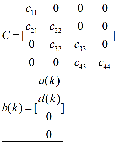
Let a(k) be the number of new freshmen admitted in the spring of year k for the following year k + 1, and let d(k) be the number of transfers into the following year’s sophomore class. Then the model becomes:

Here we have written the coefficients c21, c22, and so on in symbolic, rather than numerical, form so that we can change their values if desired.
This model can be represented graphically by a state transition diagram, like the one shown in Figure in this slide. Such diagrams are widely used to represent time-dependent and probabilistic processes. The arrows indicate how the model’s calculations are updated for each new year. The enrollment at year k is described completely by the values of x1(k), x2(k), x3(k), and x4(k), that is, by the vector x(k), which is called the state vector. The elements of the state vector are the state variables. The state transition diagram shows how the new values of the state variables depend on both the previous values and the inputs a(k) and d(k).

The four equations can be written in the following matrix form:

Suppose that the initial total enrollment of 1480 consists of 500 freshmen, 400 sophomores, 300 juniors, and 280 seniors. The college wants to study, over a 10-year period, the effects of increasing admissions by 100 each year and transfers by 50 each year until the total enrollment reaches 4000; then admissions and transfers will be held constant. Thus the admissions and transfers for the next 10 years are given by:

for k =1, 2, 3, . . . until the college’s total enrollment reaches 4000; then admissions and transfers are held constant at the previous year’s levels. We cannot determine when this event will occur without doing a simulation. I have written a pseudocode for solving this problem. The enrollment matrix E is a 4 x 10 matrix whose columns represent the enrollment in each year. The pseudocode is as follows:
Enter the coefficient matrix C and the initial enrollment vector x.
Enter the initial admissions and transfers, a(1) and d(1).
Set the first column of the enrollment matrix E equal to x.
Loop over years 2 to 10.
-If the total enrollment is <= 4000, increase admissions by 100 and transfers by 50 each year.
-If the total enrollment is > 4000, hold admissions and transfers constant.
-Update the vector x, using x = Cx + b.
-Update the enrollment matrix E by adding another column composed of x.
End of the loop over years 2 to 10.
Plot the results.
Script
% Script le enroll1.m. Computes college enrollment.
% Model’s coef cients.
>> C = [0.1,0,0,0;0.75,0.05,0,0;0,0.9,0.05,0;0,0,0.9,0.05];
% Initial enrollment vector.
>> x = [500;400;300;280];
% Initial admissions and transfers.
>> a(1) = 1000; d(1) = 200;
% E is the 4 x 10 enrollment matrix.
>> E(:,1) = x;
% Loop over years 2 to 10.
for k = 2:10
% The following describes the admissions
% and transfer policies.
if sum(x) <= 4000
% Increase admissions and transfers.
a(k) = 900+100*k;
d(k) = 150+50*k;
else
% Hold admissions and transfers constant.
a(k) = a(k-1);
d(k) = d(k-1);
end
% Update enrollment matrix.
b = [a(k);d(k);0;0];
x = C*x+b;
E(:,k) = x;
end
% Plot the results.
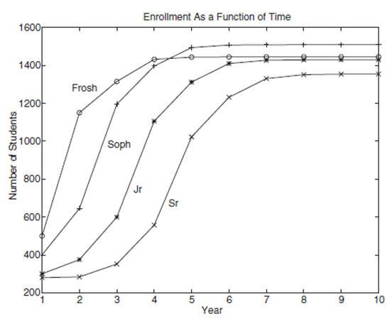
plot(E’),hold,plot(E(1,:),’o’),plot(E(2,:),’+’),plot(E(3,:),’*’),...
plot(E(4,:),’x’),xlabel(‘Year’),ylabel(‘Number of Students’),...
gtext(‘Frosh’),gtext(‘Soph’),gtext(‘Jr’),gtext(‘Sr’),...
title(‘Enrollment as a Function of Time’)
Output
The resulting plot looks something like the image below. Note that after year 4 there are more sophomores than freshmen. The reason is that the increasing transfer rate eventually overcomes the effect of the increasing admission rate. In actual practice this program would be run many times to analyze the effects of different admissions and transfer policies and to examine what happens if different values are used for the coefficients in the matrix C (indicating different dropout and repeat rates).